Foreword
After a summer hiatus, I am looking to continue to put into words many of my experiences and the lessons learned in my industrial hygiene career to date. This article covers the challenges in correcting real-time respirable dust measurements to real-time respirable silica. The first article covered in this series was the “Misnomer of Total Dust”. The second article dealt with “Carbon Monoxide in All the Wrong Places”. The third was titled “PIDs: Lamps and Response and Electron Volts…Oh My!”. A mentor of mine that has done this work a lot longer than I have has always said, “you don’t own the experience and knowledge your career has allowed you, you owe it to others“. I agree with that sentiment, as the only true way to advance the industrial hygiene profession is through the sharing of knowledge. As such, may I introduce the fourth part in my misconceptions series, “Are you Sure Your Real-time Respirable Silica Correction Factor is Correct?“. I know it is a mouthful (catchy industrial hygiene-related titles are hard to come by), but I hope that the information presented within this article helps people in the field with their real-time endeavors.
Are you Sure Your Real-time Respirable Silica Correction Factor is Correct?
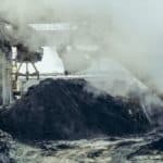
The use of real-time aerosol monitors has been gaining in popularity in recent years. The recently implemented OSHA Rule on respirable crystalline silica (1910.1053) has definitely played a part, as conversations abound in industries impacted by the standard. I have been witness to the increased interest in such tools with regards to the metal-casting industry. A typical foundry contains multiple source and fugitive exposure sources of respirable silica. These sources can range from mold-making and core-making, to shakeout, casting cleaning, conveyor systems, muller systems, ladle/furnace re-lining, etc. Simple 8-hour compliance sampling doesn’t provide the information needed to readily correct exposures exceeding the Action Level and Permissible Exposure Limit. Segmented sampling is an option, though still limited in precision (even the higher-flow options still require significant run-time) and costly (sample analysis typically runs $80 or more per sample). As such, real-time instrumentation is an appealing resource in the determination of exposure for affected employees.
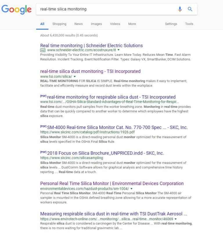
A simple google search for “real-time silica monitoring” predictably returns a huge amount of information. At the top of the search are many of the companies that you would expect….TSI and SKC both have offered real-time aerosol monitors for years. However, that first page returns lines such as:
“Personal Real-time Silica Monitor”
“real-time monitoring for respirable silica dust”
“Measuring respirable silica dust in real-time”
All of these statements stretch the definition of what real-time monitoring is. Each of these monitors can measure respirable dust in real-time. None of the monitors can directly measure respirable crystalline silica. The data can only be “corrected” to respirable silica using a correction factor. Most often, this is a %silica number from one or more filter cassette samples. Divide your real-time respirable dust average into the silica result for in-line cassette (or area/breathing zone sample) and you have a correction factor.
A Generic Correction Factor Example
Correction factors have scientific merit to them, as long as they are applied appropriately. A simple example of what this type of correction is doing can be demonstrated through the following example. Lets say you have a group of different height and weight people (see below). Some members of our cohort are tall, some are short, some are light, some are heavy.
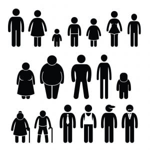
For this example, lets use height and weight as stand-ins for respirable dust and respirable silica:
Height = Respirable Dust
Weight = Respirable Crystalline Silica
With a correction factor (the total weight of the entire group), you could advertise a simple ruler to be a means of determining weight for each person. If the average height of our stick figures above was 60″, and you knew the average weight (total weight / # of people) to be 150 pounds, that would yield a correction factor of 2.5 pounds/inch. A 70″ man would weigh 175 pounds using this correction, which seems reasonable (in fact this is quite close to my height and weight). So the calculation works for an average individual. How about a 30″ child? The same correction yields 75 pounds, which is way too heavy (that would be a very large toddler). The stout man in the middle who is 74″ tall would weigh 185 pounds, which obviously underestimates his actual weight.
Applying the Height/Weight Example to a Foundry
This is the danger with correction factors. Using averages to obtain data to correct real-time data can lead to over and under-estimating the true concentrations. Consider a similar example, but now instead of simple heights/weights of a group of people, lets consider %silica content of dust found within a ferrous foundry. Silica sand is a high-use material in many foundries, so it is inherently present throughout many activities. Silica sand can be handled/dispersed when handling scrap in charging, when making molds and cores, when shaking out the solid castings, and when handling/recycling spent sand. It also burns into the surface of the casting, resulting in exposures during any subsequent finishing activity. In my experience, the respirable dust concentrations and %silica contained within that dust varies significantly throughout foundries:
1. Melting scrap produces a high respirable dust concentration (mostly metal fume/smoke) with a typically low %silica. Referencing the generic example, this would correlate to a very tall, very skinny basketball player.
2. Finishing activities such as grinding are typically the opposite, with controls that often result in low respirable dust concentrations but with a higher %silica (like a chubby infant).
3. Some shakeout and knockoff areas have very high concentrations of both…with %silica concentrations that can exceed 25% (think Andre the Giant)
It would be foolish to correlate heights to weights using whole-cohort averages for such a diverse group of individuals (a basketball player, chubby infant, and Andre the Giant). Certainly a correction factor obtained for %silica across wildly very different exposure profile processes would yield similar uncertainties.
Correction Factors during Mapping
This huge variability creates significant uncertainties when correcting real-time results. Lets say you perform a mapping activity at your facility where you measure respirable dust concentrations using a real-time monitor at hundreds of locations. Processing these results through a mapping program yields the below respirable particulate map.
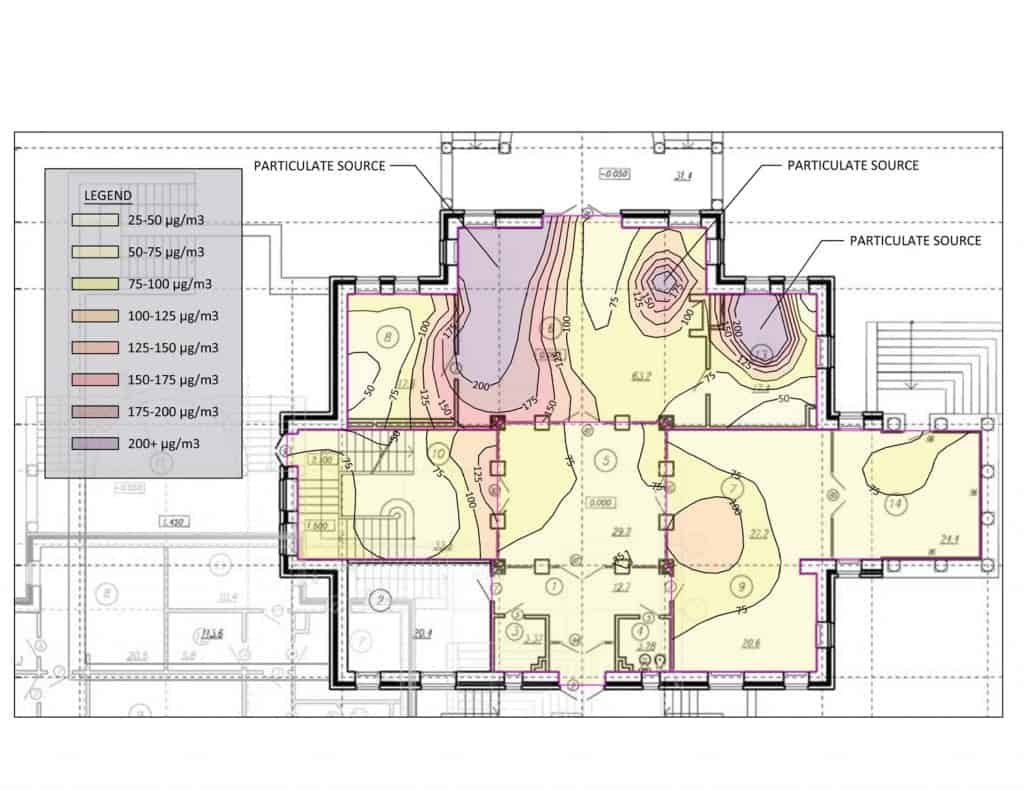
It would sure be nice to also create a map showing respirable crystalline silica numbers instead of just dust. But how can one do this?
Using the in-line filter in your real-time monitor can correct your results, but this is repeating the height/weight fallacy described earlier. You will accurately describe some areas (the ones that just so happen to align with average numbers), while significantly underestimating the silica in the short, stout areas (finishing) and overestimating the silica in the tall, skinny areas (melt). Using historical personal sampling data and area sample is more ideal (as you’ll have many corrections instead of just one), but these still are averages, 480 minute numbers in comparison to your snapshot contour map.
Correction Factors during Real-time Personal Breathing Zone Monitoring
The issue with average correction factors skewing results also arises when using such data to correct real-time breathing zone data to respirable silica. In this style of monitoring, an instrument (or its inlet) is positioned within an employee’s breathing zone, and logs concentration data at regular intervals. This can yield a real-time exposure curve, like the example shown below.
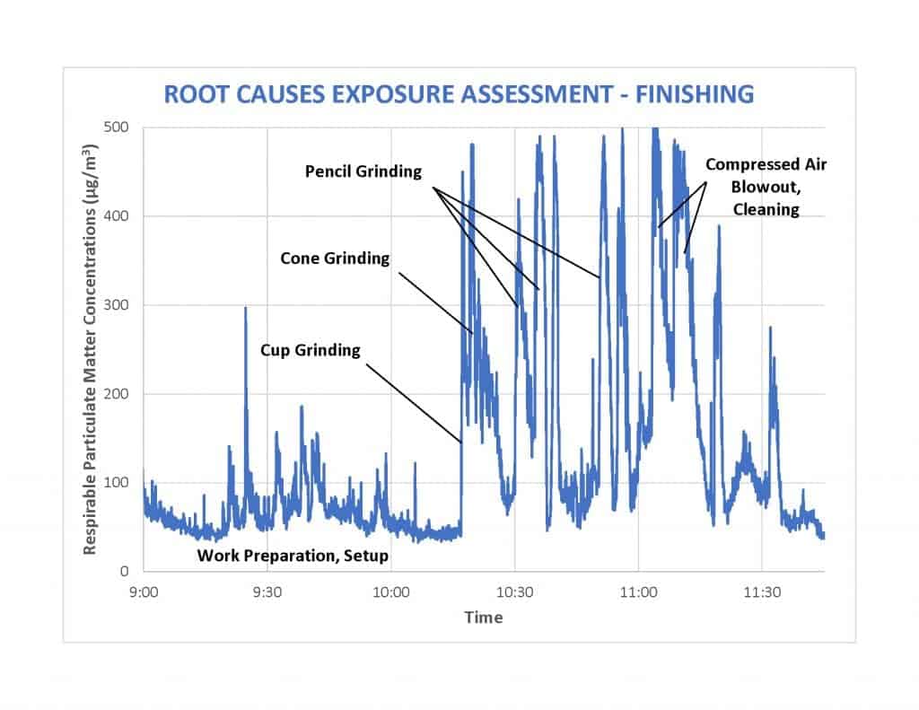
A similar issue arises when correcting these results to %silica. Using average data will overestimate some exposures while underestimating others. Perhaps that pencil grinding activity happens to take place on pocket of the casting with huge amounts of residual/burnt-in sand. Maybe the compressed air exposures are a result of non-respirable silica sources dispersed from the booth floor. There is no way to determine which is which through the average data provided by a sample cassette that generates the correction factor.
Some Recommendations Regarding Correction Factors
Everything I described up until this point paints a bleak picture for the use of correction factors to obtain respirable silica results from real-time respirable particulate data. My own path to this knowledge has been long and winding, encompassing hundreds of hours of boots-on-the-ground real-time monitoring and the processing of results. I can assure you that all is not lost however! With enough foresight, one can get closer to an acceptable level of accuracy. My advice regarding the collection of real-time monitoring data for the purpose of correcting to real-time silica is as follows:
1. Do not mix process types – Keep each set of real-time measurements to the same type of process. When you measure melt, generate a correction factor for just melt. Do not proceed to measure mold-making and finishing departments on the same cassette.
2. Consider the sample duration – Ensure the duration of each real-time measurement set is as short as possible. Longer duration measurements will result in higher uncertainties when correcting real-time results. (This can be tricky, as you need to ensure you are obtaining sufficient material to exceed laboratory detection limits).
3. Consider the use of ranges – I highly recommend communicating the uncertainty with the corrections using ranges instead of static results. Why say that the real-time average exposure generated during a compressed air blow-off task is 45.6 micrograms per cubic meter, when you certainly don’t have the confidence to state it as such. With sufficient data, you could say such a task ranges from 40-60 micrograms per cubic meter, which more effectively incorporates the error inherent to this process.
4. Learn your instruments! – Each real-time aerosol monitor has its own quirks, which can influence results. There are some models that recirculate sheath air to the sensor, resulting in a corrected volume to the cassette (you will be way off if you don’t account for this).
5. Use caution with historical data – Conditions change over time based upon a huge number of variable conditions (temperature, fugitive processes, overhead doors, alloys, etc.). Using historical data thus presents its own uncertainties.
5. Even simultaneous personal sample has flaws – Anyone that has performed side-by-side sampling during an OSHA audit knows that results rarely agree with one another. Putting a sample pump/cyclone on one shoulder and a real-time monitor on the other could measure significantly different conditions and be subject to variable error.
Summary
The more data you have, the better you will understand the variability and errors that are associated with real-time monitoring. As such, I’d recommend generating dozens of corrections over time rather than just a one or two. Like everything within industrial hygiene, this technology is a tool, that if used correctly, can shed light on information that previously remained hidden. These instruments are terrific qualitative resources, measuring the magnitude of exposures and pinpointing locations where engineering controls can be deployed. The instruments are less useful quantitatively, but only because of the limitations of the correction factor.
In summary, just because an instrument has limitations does not mean it is unusable. Most instruments have flaws, the key is to understand them, and act appropriately. Understanding the errors associated with data can be just as important as the data itself!